On-Sky Testing of the NASA42 Camera
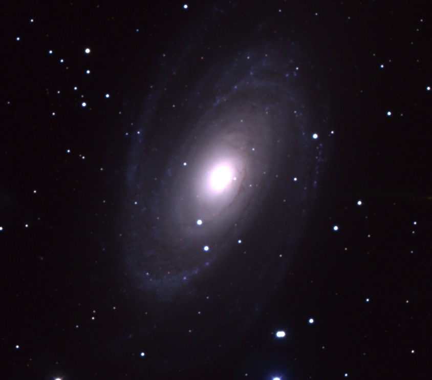
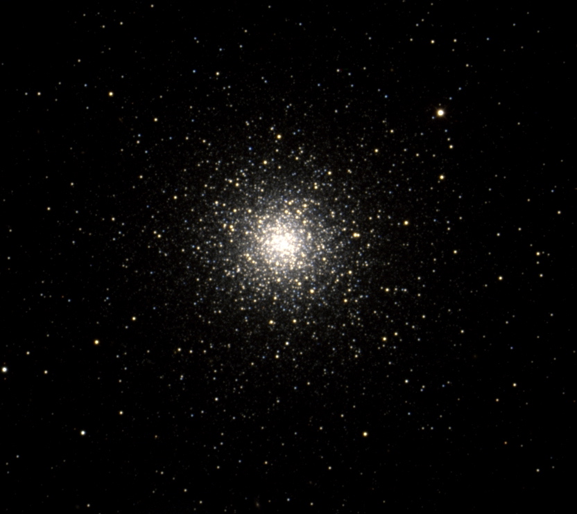
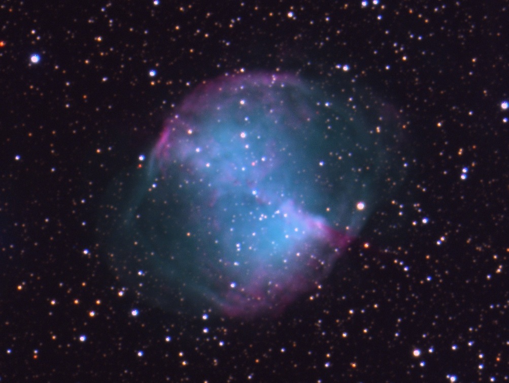

Images of M81,M3,M27 and M51 obtained with NASA42 Camera by Kathryn Neugent
This summarizes the results of the on-sky testing by Kathryn Neugent and Phil Massey after Ted adjusted the operating voltages of the NASA42 Camera chip in order to improve the linearity. Specifically we wanted to perform the following tests:
The final voltages were achieved by Ted on May 10th, and we conducted our tests on May 11th, a photometric night but one mared by poor and variable seeing.
We measured the gain and read-noise for Amplifier A (the default single amp readout) using Janesick's method on pairs of dome flats and biases, restricting the sample to the middle 200x200 section. We obtained values of the gain of 3.71-3.78 e/ADU, and values for the read-noise of 4.27-4.35 e-. Using a full-blown analysis Ted finds 3.84e/ADU and a readnoise of 4.6 e-. So, reasonably solid values are 3.8 e/ADU and 4.5 e-.
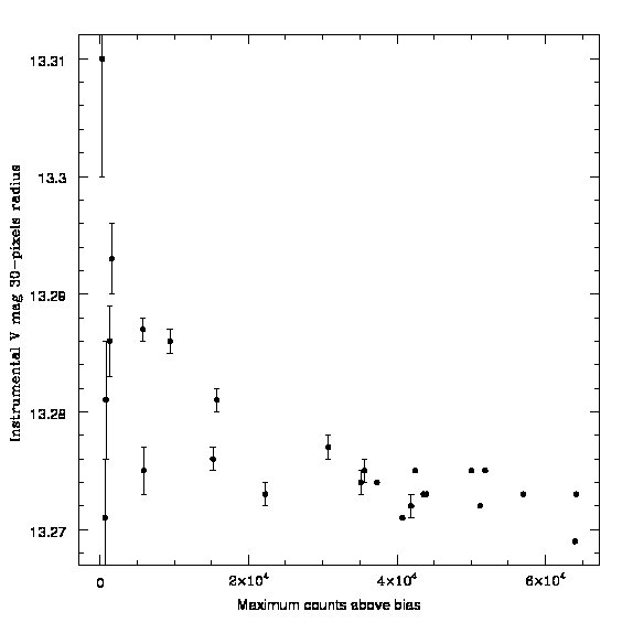
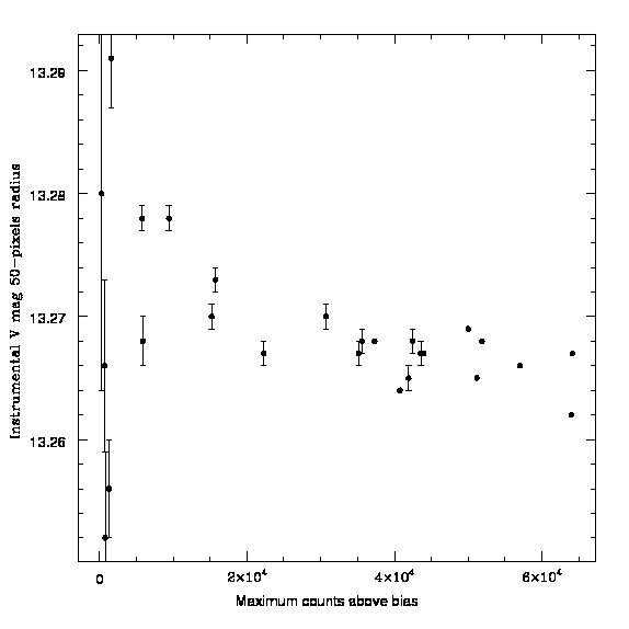
We took a series of 26 exposures of a (random) star near zenith. The exposure times ranged from 0.2 to 50 seconds, with a resulting peak count rate of 280 to 64,000+ above bias (roughly 1632), i.e., taking it right up to the 65,535 range of the A-to-D converter.
Because the seeing was so bad (fwhm 4.5-7.5 pixels) we used measuring radii of 30 and 50 on the star. Our results are shown in the two plots (left = 30, right = 50). As far as the stellar photometry is concerned, there is no sign of any non-linearity over the full range of the A-to-D converter.
We took a series of exposures of the dome flat through each broad-band filter, and also exposures of the "uniformally illuminated" twilight spot shortly after sunset. There was a clear gradient from left to right on the images, amounting to about 4%, with the twilight having more counts on the left. Which (if either?) is right?
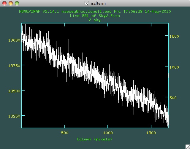
We answered that definatively by simply moving a (random) star around the field. Using twilight skies as the flats gave consistent photometry to <1%; the photometry based on flattening by the dome flats varied by 4% depending upon location of the star in the field.
u-U=5.19-0.09(U-B)
b-B=3.62+0.00(B-V)
v-V=3.34+0.01(B-V)
r-R=3.21-01(v-R)
The color terms are all negligible except for a modest term at U, due primarily to the filter. We did find a horrendously large color term for the I filter, to the extent that we don't believe the results. We will remeasure it.
| U | B | V | R |
|---|---|---|---|
| 3.19 | 17.2 | 17.5 | 19.8 |
Coming Soon!